This page documents a few aspects of memory management on Java containers on K8s clusters.
For java containers, memory management on K8s have various factors:
Xmx and Xms limits managed by java
Request/limit values for the container
HPA policies used for scaling the number of pods
Misconfigurations / misunderstanding of any of these parameters leads to OOMs of java containers on K8s clusters.
Memory management on java containers:
-XX:+UseContainerSupport is enabled by default form java 10+
-XX:MaxRAMPercentage is the jvm parameter that specifies the percentage value of limits memory defined on the container, that can be used by heapspace. Default value is 25%.
Example: if -XX:MaxRAMPercentage=75, and container memory limit is3GB, then:
-Xmx=75% of 3GB = 2.25GB
Important point to note: MaxRAMPercentage is calculated on limits and not requests
K8s : requests/limits:
as shown above, the memory assignment for the container is based on the values set for limits configuration
However, for hpa to kick-in, requests is used for Kubernetes.
Example:
If you configure HPA for memory utilization at 70%, it calculates usage as:
scaling would happen usage wrt request configuration
If requests.memory is set low (2GB) and limits.memory is high (3GB), HPA may scale aggressively because it calculates usage based on requests, not limits.
The only advantage of setting limit > request – is : if non-heap space growth increases, it will not crash the vm. That’s one of a case with less probability compare to heap space crash.
Ideally, to make things simpler, based on the historic usage of the application – set “request=limits” for memory usage on java container. This will simplify the Xmx, request, limits and hpa math.
For scaling apps, there is alway HPA which can increase instances based on usage.
Conclusion
for java containers on K8s, know the memory needs of your app and set “request=limits”
use hpa for scaling and not depend on “limits>request” for memory
containers: run them small and run them many (via scaling based on rules)
In this write up, we will try and explore how to make the most out of the resources in K8s cluster for the Pods on them.
Resource Types:
When it comes to resources on Kubernetes cluster, they can be fairly divided in to two categories:
compressible:
If the usage of this resource for an application goes beyond the max, it can be throttled without directly killing the application/process.
example : cpu – if a container consumes too much of compressible resource, they are throttled
non-compressible:
If the usage of this resource goes beyond max, it cannot be directly throttled. Might lead to killing of process.
example : memory – if a container consumes too much of non-compressible resource, they are killed.
For each pod on a k8s, there are mainly 4 types of resources which need tuned and management based on the application running: CPU, Memory, Ephermal-storage, Hugepage-<size>
Each of the above mentioned resource can be managed at Provisioning level and Cap usage level on K8s. That is where requests/limits in K8s come in handy.
Request/Limits:
Requests and Limits are the important part of Resource management for Pods and containers.
Requests: is where you define how much of resource your pod needs, when it is getting scheduled on worker node. Limits: is where you define what is the max value that the resource can stretch to, when consuming the resource on worker node.
Lets consider the deployment yaml file for a application which has request/limit defined on cpu and memory. It is important to note that when a pod is provisioned on a worker node by kubernetes scheduler, the value mentioned in requests is taken into consideration. The worker node needs to have the amount resource described in requests field for the pod to be scheduled successfully
At a high level, the concept of requests/limits is similar to soft/hard limits for resource consumption. (more like xms/xmx in Java). These values are generally defined in the deployment file for the pod. It is an option to either set Request/Limits individually or skip them altogether(based on the kind of resource). If the requests and limits are set incorrectly, this could lead various issues like:
pod instability
workers being underused
incorrect configuration for compressible and non-compressible resources.
worker nodes being over-committed.
affecting directly the quality of service for a pod (Burstable, Best-Effort, Guaranted)
Now lets try and fit in different Requests/Limit metrics for CPU and Memory resources for an application deployed on K8s cluster
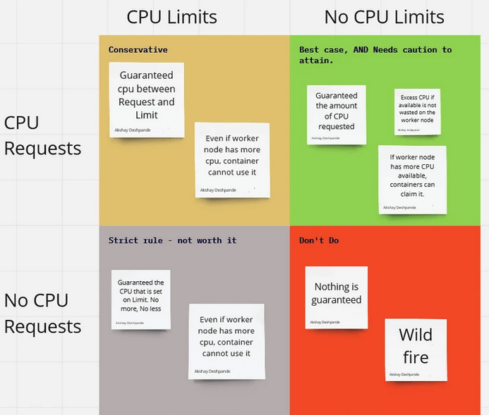
CPU :
CPU is a compressible resource – can be throttled.
It is an option to NOT set Limit on CPU. In that case, if there is more CPU available on the worker note, unused, the pods without limits can over-commmit and use the available CPU.
It is an option to not set Limit for resources which are compressible, because they can be throttled when there is worker needs the memory back.
If your application needs guaranteed Quality of Service, then set the Request==Limit
Below is general plot of Request/Limits for CPU
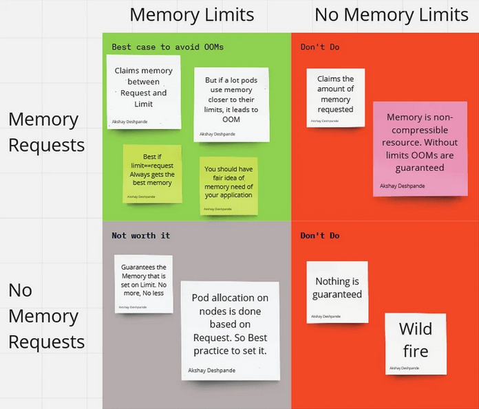
Memory :
Memory is a non-compressible resource – cannot be throttled. If a container uses more memory, it will be killed by the kubelet.
You cannot ignore Limits like in CPU resource because when the memory need of the app increases, it will over-commit and affect the worker node.
Values for limits and requests based on the application needs and tuned based on production feedback of the container.
If your application needs guaranteed Quality of Service, then set the Request==Limit
This writeup is more of a demo to showcase the power of “proc” (process information pseudo-filesystem) interface in linux to get the memory details of process, and also a quick brief on the power of “proc interface”.
In the current trend of building abstraction over abstractions in software/tooling, very few tend to care about the source of truth of a metrics. There are various APM / Monitoring tools to get the memory details of a process for a linux system, but when the need arises, I believe, one must know the ways of going closer to the source of truth on a linux system and verify things.
So, What is proc ?
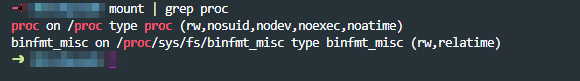
proc stands for “process information pseudo-filesystem.” proc is a pseudo-filesystem that provides an interface to the Linux kernel. It is generally mounted at /proc and is mounted automatically by the system.
listing mounts
As seen above, on listing the mounts, you can see the device proc, which is not really a device, but is just the listed as word proc meaning that it’s a kernel interface.
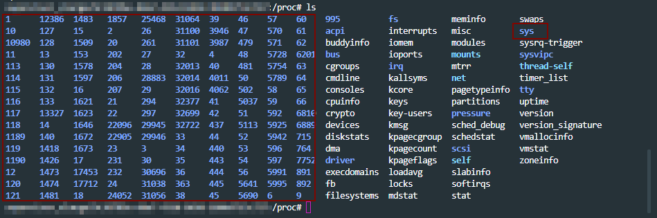
In proc, you can see three different categories of information mainly.
sys directory – has details for files, kernel, networking, virtual memory etc of the system.
pid directories – which contains details of what a process is doing at process level.
status files like – cpuinfo, meminfo etc of the system.
a look into /proc path. pids, sys highlighted. Rest are status files.
A lot of the linux toolings like ps get the process level information from /proc path. An overview of proc at the man page – here
With that general overview of proc interface, let move to getting memory information for a process in detail for our use case.
Scenario: A java process is crash periodically and consistently. How to get the memory details for the pid using /proc interface ?
To begin with, there are more than one ways of doing this analysis. For example: set up auto dump generators on heap(JVM params) and set up the core dump generation on ulimit. Get the dumps on crash and work backwards by analyzing them.
Since the intention here is to discover the capabilities of /prod/pid/* tooling, we will try and collect metrics from these toolings for our analysis.
First, lets collect the metrics for the java process running on the system from the /proc directory as the java process is running, so that we can analyze it. A tiny shell script for that below.
ps = "java";
seconds = "60";
dir = "memstats";
while sleep
  $seconds;
do
  ts = "$(date +'%F-%T' | tr : -)";
echo "Collecting memory statistics for process(es) '$ps' at timestamp '$ts'";
for pid
  in $ (pidof $ps);
do
  echo "- Process ID: $pid";
pdir = "$dir/$ps/$ts/$pid";
mkdir - p $pdir;
cp / proc / $pid /
{
maps, numa_maps, smaps, smaps_rollup, status}
$pdir /;
done;
done
The above script: – creates the directory structure – monitors the running java processes every 60secs – copies the /proc/$pid metrics dump to the above directory structure
Let the above script run and collect the metrics, as the java process we are monitoring is getting to crash. Once we have the metrics collected, lets look in to the memory details of the pid crashing.
metrics collected before the process crashed from above script
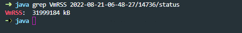
The system under test had 32 GB memory in my case.
If we look at the vmRSS memory for the process dump, we see that java process is consuming all 32GB of the memory. Notice that status file is looked in to from /proc/pid which has the memory usage details for the process.
This is reflected closely by the sum of Rss values of each VM area/section collected in above dump. Note that we are digging in to smaps from /proc/pid to get these details on each VM section here for cross validation.
One observations on object sizes is, the VMAs with RSS on 10 MB or more (5 or more digits for kB field) are 429, which we get by looking in to smaps for the pid.
Before the next observation, look at one of the entires of an object in smaps file.
details of one of the objects in smaps file. Similar details for each object will be present in the smaps file.
smaps file for the pid in /proc has a lot of details about the residing objects which are consuming the memory. Going back to the objects of size more than 10MB, all 429 objects don’t have any file reference which were holding the memory in my case, and the allocation was Anonymous. (refer to Anonymous row in the above image)
we are trying to get all the objects which are over 10MB, and have a file reference to them. We get zero such files.
“Anonymous” shows the amount of memory that does not belong to any file. More details on Anonymous reference on the kernel documentation here
In short, what the above data points infer is, for the java process which is crashing, all the size does not come from jvm heap but comes from non-java / C-style allocation. Most probably the crash is happening JNI layer.
In such cases, you will not even see any heap dump getting generated. However, core dumps will be generated as diagnostic dumps for analysis if the “core file size” is set to unlimited in “ulimit“. More details on how to get core dumps here .
With the above details, this might be due an internal library which is used in the application which is non-java and is causing the crash.
From here you can look at “maps” file under “/proc/$pid/” to look at all the non ".jar” files to look at the non-java references and analyze it further.
In my case, it was a bunch of non-standard libraries which were packaged, that was causing the crash in JNI layer. Updating which solved the issue.
Conclusion:
There are always more than one ways of solving the problem.
The purpose of this write up again, was to show the power of understanding linux process diagnostics that come with built in with "/proc” interface.
Building abstractions and not letting ssh access to vms (which is the current industry trend) is great, but going closer to the source of truth can help solve problem sometimes when you know what you are looking for.
As a Performance Engineer, time and again you will come across a situation where you want to profile CPU of a system. The reasons might be many; like, CPU usage being high, you want to trace a method to see its CPU cost or you suspect CPU times for a slow transaction.
You might use one of the various profilers out there to do this. (I use yourkit and Jprofiler). All these profilers report the CPU costs in terms of CPU Time, when you profile the CPU. This time is not the equivalent of your watch time.
So in this article, let’s try and understand what is CPU time and other fundamentals w.r.t to CPU.
Clock Cycle of CPU :
The speed of a CPU is determined by its clock cycle, which is the amount of time taken for one complete oscillation of a CPU. (which is two pulses of an oscillation). In more simple terms, consider your CPU like a pendulum. It has to go through it’s 0’s and 1’s, i.e, rising edge and falling edge. The amount of time taken for this one oscillation is the Clock Cycle of a CPU. Each CPU instruction might take one or more CPU cycles to execute.
Clock speed (or Clock rate):
This is the total number of Clock cycles that a CPU can perform in one second. Each CPU executes at a particular clock rate. In fact, Clock speed is often marketed as the primary capacity feature of a processor. A 4GHz CPU can perform 4 billion Clock Cycles per second.
Some processors are able to vary their clock rates. Increase it to improve performance or decrease it to reduce power consumption.
Cycles per instruction (CPI) :
As we know, all the requests are served by CPU in the form of instruction sets. A single request can translated in to 100’s of instruction sets. Cycles spent per instruction is an important parameter which helps understand where CPU is spending its clock cycles. This metrics can also be expressed in the inverse form, i.e, Instructions per Cycle (IPC).
It is important to note that CPI value signifies the efficiency of instruction processing , but not of the instructions themselves.
CPU Time :
After knowing the above parameters, it is much easier to understand CPU time for a program now.
A single program will have a set of Instructions. (Instructions / Program) Each instruction will consume a set of CPU cycles. ( Cycles / Instruction ) Each CPU cycle is based on the CPU’s clock speed ( secs / cycle)
Hence, the CPU time that you see in your profiler is :
CPU Time for a process = (No. of instructions executed) X (Cycles per Instruction) X Clock Cycle.
So the next time when you see “Time” being mentioned in your Profiler, remember the above calculations. Happy tuning.
These are the self-notes from managing 100+ node ES cluster, reading through various resources and a lot of production incidents due to unhealthy ES.
Memory
Always choose ES_HEAP_SIZE 50% of the total available memory. Sorting and aggregations both can be memory hungry, so enough heap space to accommodate these is required. This property is set inside the /etc/init.d/elasticsearch file.
A machine with 64 GB of RAM is ideal; however, 32 GB and 16 GB machines are also common. Less than 8 GB tends to be counterproductive (you end up needing smaller machines), and greater than 64 GB has problems in pointer compression.
CPU
Choose a modern processor with multiple cores. If you need to choose between faster CPUs or more cores, choose more cores. The extra concurrency that multiple cores offer will far outweigh a slightly faster clock speed. The number of threads is dependent on the number of cores. The more cores you have, the more threads you get for indexing, searching, merging, bulk, or other operations.
Disks
If you can afford SSDs, they are far superior to any spinning media. SSD-backed nodes see boosts in both querying and indexing performance.
Avoid network-attached storage (NAS) to store data.
Network
The faster the network you have, the more performance you will get in a distributed system. Low latency helps to ensure that nodes communicate easily, while a high bandwidth helps in shard movement and recovery.
Avoid clusters that span multiple data centers even if the data centers are collocated in close proximity. Definitely avoid clusters that span large geographic distances.
General consideration
It is better to prefer medium-to-large boxes. Avoid small machines because you don’t want to manage a cluster with a thousand nodes, and the overhead of simply running Elasticsearch is more apparent on such small boxes.
Always use a Java version greater than JDK1.7 Update 55 from Oracle and avoid using Open JDK.
A master node does not require much resources. In a cluster with 2 Terabytes of data having 100s of indexes, 2 GB of RAM, 1 Core CPU, and 10 GB of disk space is good enough for the master nodes. In the same scenario, the client nodes with 8 GB of RAM each and 2 Core CPUs is a very good configuration to handle millions of requests. The configuration of data nodes is completely dependent on the speed of indexing, the type of queries, and aggregations. However, they usually need very high configurations such as 64 GB of RAM and 8 Core CPUs.
Some other important configuration changes
Assign Names: Assign the cluster name and node name.
Assign Paths: Assign the log path and data path.
Recovery Settings: Avoid shard shuffles during recovery. The recovery throttling section should be tweaked in large clusters only; otherwise, it comes with very good defaults. Disable the deletion of all the indices by a single command: action.disable_delete_all_indices: false
Ensure by setting the following property that you do not run more than one Elasticsearch instance from a single installation: max_local_storage_nodes: “1” Disable HTTP requests on all the data and master nodes in the following way: http.enabled: false
Plugins installations: Always prefer to install the compatible plugin version according to the Elasticsearch version you are using and after the installation of the plugin, do not forget to restart the node.
Avoid storing Marvel indexes in the production cluster.
Clear the cache if the heap fills up when the node start-up and shards refuse to get initialized after going into red state This can be done by executing the following command:
When you come across a system which is misbehaving, majority of the times the first metrics that we look at is CPU usage. But do we really understand what CPU usage of a system tells us ? In this article let us try and understand what X % usage of a system really means.
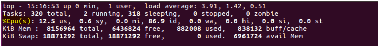
One of the easy ways to check on CPU is “top” command.
The “%Cpu(s)” metrics seen above is a combination of different components.
us – Time spent in user space
sy – Time spent in kernel space
ni – Time spent running niced user processes (User defined priority)
id – Time spent in idle operations
wa – Time spent on waiting on IO peripherals (eg. disk)
hi – Time spent handling hardware interrupt routines. (Whenever a peripheral unit want attention form the CPU, it literally pulls a line, to signal the CPU to service it)
si – Time spent handling software interrupt routines. (a piece of code, calls an interrupt routine…)
st – Time spent on involuntary waits by virtual cpu while hypervisor is servicing another processor (stolen from a virtual machine)
Out of all the breakdowns above, we usually concentrate mainly on User Time (us) , System time(sy) and IO wait time (wa). User time is the percentage of time the CPU is executing the application code and System time is the percentage of time the CPU is executing the kernel code. It is important to note that System time is related to application time; if application performs IO for example, the kernel will execute the code to read file from disk. Also, any wait seen in IO will reflect in IO wait time. So us%, sy% and wa % are related.
Now let’s see if we understand this correctly on a whole.
My goal as a Performance Engineer would be to drive the CPU usage as high as possible for as short a time as possible. Does that sound far away from the “best-practice” ? Wait, hold your thought there.
The first thing to know is, the CPU usage reported by any command is always an average over an interval of time. If the CPU consumed by an application is 30% for 10minutes, the code can be tuned to make it consume 60% for 5minutes. Do you see what I mean by “driving the CPU as high as possible for as short time as possible”? This is doubling the performance. Did the CPU usage increase ? Sure, Yes. But is that a bad thing ? No. CPU is sitting there waiting to be used. Use it, improve the performance. High CPU usage is not a bad thing all the time. It may just mean that your system is used at its full potential. A good ROI. However, if you have your run-queue length increasing, where requests are waiting for cpu, then it definitely needs your attention.
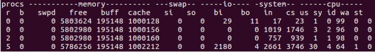
In linux systems, the number of threads that are able to run (i.e, not blocked on IO or sleeping etc) are referred to as run-queue. You can check this by running “vmstat 1” command. The first number in each line refers to run-queue.
If the count of the threads in the above output is more than the available CPU’s (count in hyper-threading if enabled), that means the threads are waiting for CPU and the performance will be less the optimal. Although a higher number is ok for a brief amount of time, but if the run-queue length is high for a significant amount of time, it is an indication that system is overloaded.
Conclusion :
High CPU usage of a system is not a bad sign all the time. CPU is available to be used. Use it and improve the performance of the running application.
If run-queue length is high for a significant amount of time, that mean the system is overloaded, and needs optimizations.
In this world of Microservices and the distributed systems, a single request (generally) hops through multiple servers before being served. More often than not, these hops are also across the Network cards making the Network Performance the source of slowness in the application. These parameters makes the need to measure Network performance between servers/systems more critical for benchmarking or debugging.
Iperf3 is one of the open source tools which can be used for network throughput measurement. Below are some of its features.
Iperf3 can be used for testing maximum TCP and UDP throughput between two servers.
Iperf3 tests can also be run in a controlled to way to not test the maximum limits but ingest and constant lower network traffic for testing.
Iperf3 has options for parallel mode(-P) where multiple clients can be used, setting CPU affinity(-A), pausing certain intervals between two requests(-i), setting the length of buffer to read or write(-l), setting target bandwidth (-b) etc.
More important than anything is the fact that iperf3 runs as an independent tool outside your application code. The results from this tool removes any ambiguities/doubts on the application code which might be causing the network problems.
Installation of iperf3 tool:
sudo apt-get install iperf3
iperf3 tool has be installed on both servers between which you want to measure the network performance. One of the machines is treated as client and other as server.
Command to run on the server:
Below command when run on one of the two servers under test, signifies that the machine is acting as a server for the iperf test.
iperf3 -s -f K
-s — runs in server mode
-f K — signifies the format as KBytes. Note : If you do not want to use the default port (which is 5201) for the test, then specify the port with the option -p in the above command and use the same on client as well.
Command to run on the client:
Below command when run on the other server under test, pushes network bandwidth to server and reports the network capacity based on options used.
From the output (last two lines), it can be seen that the total bandwidth available between the two servers is 708MBytes/sec.
There are also various other options available for iperf3 tool. Like the below command specifies the test to be run for 60secs, which is by default 10secs (-t 60), specifies a target bandwidth of 10MB (-b 10M), number of parallel client streams set to 10 (-P 10).
Below are some of the cases where I have used iperf3 for debugging purpose:
Throughput of the application doesn’t scale but there is no obvious resource contention in cpu, memory or disk. On running “sar -n DEV 2 20” I could see network usage doesn’t peak above 30MB/sec. On using Iperf3 for benchmarking we could see 30Mb/sec was the max network capacity between the servers.
When we wanted to find the impact of vpn on the network throughput we used iperf tool for comparative analysis.
Hope this gave you a sneak peak into iperf3 tool’s capability and usages. Happy tuning!
In the previous article about Java Thread Dumps (link here) we looked in to a few basics on Thread dumps(When to take?, How to take?, Sneak peaks? etc.)
In this write up, I wanted to mention a few tools which can ease the process of collecting and analyzing thread dumps.
Collecting multiple thread dumps:
I prefer command-line over any APM tools for taking thread dumps. The best way for analyzing threads is to collect a few thread dumps (5 to 10) and look through the transition in the state of threads.
As mentioned in the previous article(link), one of the ways is using jstack, which is built in to jdk. Below command will collect 10 thread dumps with a time interval of 10sec between each. All dumps are written to a single file ThreadDump.jstack.
You can further split the 10 thread dumps to individual files using the csplit command. The below command basically looks for the line “Full thread dump OpenJDK” which is printed at the started of each thread dump and splits the dump in to individual ones.
To start with, there are many tools like VisualVM, Jprofiler, Yourkit and many more online aggregators for visualizing and analyzing ThreadDumps. Each one have their own pros & cons. Here is a small list of available tools – link
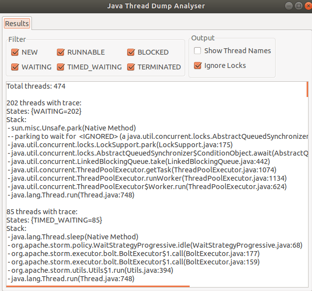
I generally use the “Java Thread Dump Analyser” (JTDA) tool from here.
This tool is available as a jar, to which you can feed the Thread dump file via command line and visualize Threads grouped in there States. You would appreciate this grouping if you have analyzed Thread Dumps in vim which had 100’s and 100’s of lines.
java -jar jtda.jar <ThreadDumpFilePath>
Here are some of the features which I like about JTDA tool:
light weight and doesn’t need any configuration.
you can upfront get the count of threads in all states
you can only look in to threads that are in a certain state (Runnable / Waiting / Blocked etc)
threads with same stack are grouped together for ease of reading
“show thread name” if checked, give the name of thread pool for better context.
On the foot note, when looking in to thread dumps, it is very important to know the code paths and the request flows. This helps in root causing the issue and better reading / understanding of thread dumps.
A few short thoughts / ideas wrt of Performance centric product.
In this world of infinite scaling of computes, pay close attention to common choke points. Like DB, storage(s) etc, which are shared by all the computes.
Majority of the reads and writes have to happen in Bulk operations and NOT as single read/writes. Specially when there are 100’s-1000’s of reads/writes/deletes on storage(s).
Threads. Pay close attention to which part of the entire flow is multi-threaded. Sometimes, only a small part of the flow is multi-threaded, but entire application is called multi-threaded, which is wrong.
Don’t just look at throughput for certifying if an application is performing good / bad. Scenario 1: Throughput:100docs/sec, Object size:100Kb Scenario 2: Throughput:50docs/sec, Object size:200Kb In both the cases about the amount of data transferred on network is 10,000Kb/sec (9.7Mb/sec). So pay attention to network stats and size of objects as well.
Databases. Make sure important collections have indexes. (There is so much more to DB tuning. This could be starting point)
Introduce local cache on computes wherever possible to avoid network calls to DB’s. Be 100% sure on your logic on when to invalidate the cache. If we don’t invalidate the cache and use the stale cached data, that could lead to incorrect transactions.
Failures are important. Pay close attention to reducing the failures. If something has to fail, then fail early on its compute cycle, so that CPU cycles are not wasted on failures.
When you do retries due to failures in your system, make sure to have logarithmic back offs. Meaning, if a message failed, 1st retry after 1min, 2nd retry after 2mins, 3rd after 4mins etc. This give system time to recover. Also retry only for finite number of times.
Pay very close attention on logic for when to mark a failure as Temporary vs Permanent. If a failure which should be permanent is wrongly marked as temporary, then the request keeps coming back to the compute via retries and wastes the CPU cycles.
Timeouts and Max connection pool sizes! Make a note of all the timeout that are set across talks between different fabrics / api calls in your application. Also, see the configuration for connections pools used in the application. Both might result in spike of failures if crossed.
[Update:]
Redundancy, Isolation and Localization are the core of any reliable system. Redundancy in the service to handle any failures. Isolation to break transactions in to independent smaller services. Localization so that you have all the required compute and data locally in the service with minimum/none external dependency.
This is first of a two parts article which talks about:
What are thread dumps?
When to take thread dumps ?
How to take thread dumps ?
What is inside a thread dumps ?
What to look for in a thread dump?
Majority of the systems today are mutlicore and hyper-threaded. Threading at the software level allows us to take advantage of a system’s mutlicores to achieve the desired pace and efficiency of the application operations. Along with pace and efficiency, multi-threading brings its own set of problems w.r.t thread contentions, thread racing, high CPU usage etc. In this write up we will see how to debug these problems by taking thread dumps on java applications.
What are thread dumps ?
A thread dump is a runtime state of a program at a particular point in time. It can also be looked at as a snapshot of all the threads that are alive on the JVM. In a mutli-threaded java application there can be 100’s of threads. Although mutli-threading improves the efficiency of an application, it makes it complex to know what is happening at a given point in the application. This is where thread dumps come in handy, which gives us a textual representation of all the thread stacks of all the threads in the application.
When to take thread dumps ?
Thread dumps can be helpful in the scenarios like: – you want to know the state of application. – you want to know if all the threads from the assigned thread pool are used and are doing work. – when you are seeing high CPU and want to see which current running threads are causing high cpu. – when you are seeing unusual slowness in the application. – with certain jvm parameters, jvm takes auto thread dumps if jvm crashes to help debugging the crash.
How to take thread dumps ?
Two easy ways of taking thread dumps are using jstack or with kill -3 command.
It is best to take a bunch of thread dumps with a slight time gap to better analyse the application. If you use jstack, you could take 10thread dumps with 10seconds sleep time between each, using below shell command. Note: replace <pid> with your process id in below command.
There is enough content available online on these. So I will link them below. – Oracle documentation on jstack link – Redhat knowledge base link – Tutorial point link – Multiple other ways link – If you are using kill -3, note that thread dumps will go to system out of JVM – link
What is inside a thread dump ?
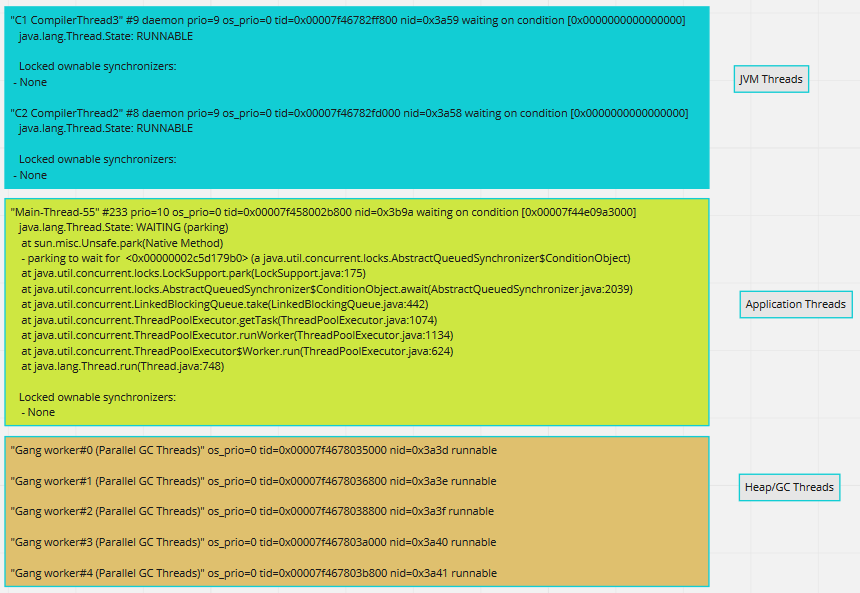
Now that we are done with boilerplate sections, lets see the main part. When you open a thread dump, you generally see three kinds of threads. JVM threads(some), Application threads(many) and Heap/GC threads(few). Snippets of these threads are shown below.
Three kinds of threads in ThreadDumps
Elements in a single thread stack:
For debugging an application, Application threads are our area of interest. When inspecting a single Application thread, it has below parts in it.
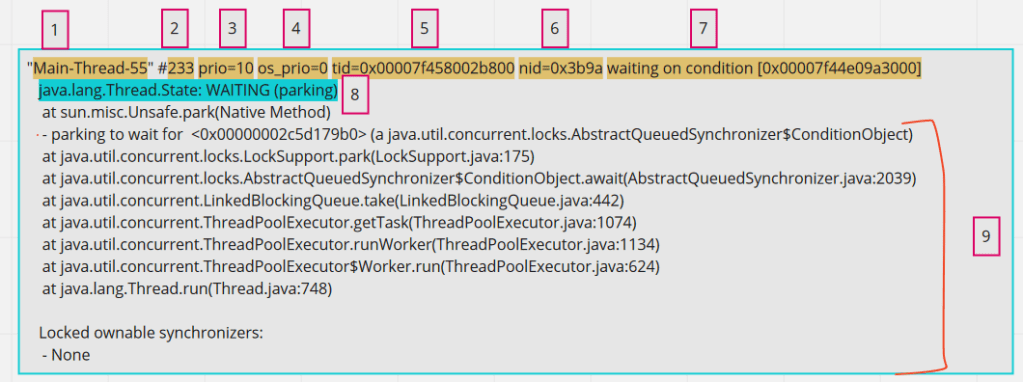
components of a single application thread
1 – Thread name, obvious and straight forward . 2 – Number id of thread. This will get incremented everytime there is a new thread created for that thread pool. 3 – JVM priority. This number signifies the priority of the thread in JVM. Java exposes api for setting thread priority. 4 – Priority of a thread on the operating system. 5 – Thread id for the thread in the memory 6 – Native thread id assigned to JVM by OS. This is important of correlating JVM threads with OS threads. 7 – This is optional seen only when the thread is waiting on some condition. May not be always. 8 – Thread state. In my opinion, this is overrated and generally over-analyzed. Reflect the current state of the thread. 9 – Thread call stack. Reads bottom-up. Gives the stack of thread.
States of a thread:
This is element [8] in the above highlighted breakdown. Below are the different states that a thread might be in.
RUNNABLE – This is the thread which is running on CPU and actively executing code.
WAITING – A threads in this state will wait indefinitely unless some other thread wakes it up. Some examples are threads which are waiting on IO or threads waiting for data to be returned from DB.
TIMED_WAITING – Similar to waiting but the thread will wake up after a specific period of time. Storm Spout threads which wake up every few seconds are a good example.
BLOCKED – Threads waiting to acquire a monitor lock. In Java, blocks of code can be marked as “synchronized”, so when a thread acquires a monitor lock, other threads will wait in this state, until the monitor is available.
NEW & TERMINATED – these states are rarely seen and are of least interest.
What to look for in a thread dump?
Now that we know most part of what can be found in a thread dump, lets see what we should be looking at for analysis.
The first important thing is to look at your application threads related info to begin with. For this, pay attention to thread name ( Element [1] in above breakdown). Obviously one would know the thread pools created by the application, and you need to look at the threads whose name belong to this Thread pool names.
Look out for the threads in RUNNABLE state amongst the above selected application threads. These are the threads which are actually doing the work and running on the cpu. Example: If a thread pool of 200 is set and if only 10 of those threads are in RUNNABLE state, then you might want to look at what rest of the 190 threads are doing.
Even in the RUNNABLE threads, it is important to see if the thread is busy executing any NATIVE methods. When you see the calls being made to Native methods in the thread dump, that means the thread is not executing Application code at that point, but is executing JNI (java native interface) code. Native methods are pre-compiled piece of codes from JVM which might be serving small specific purposes like reading from socket connections (like in below example), making file system calls etc. If you see a lot of threads in RUNNABLE state, but are busy executing Native methods, then it might not be application code issue but environment issue in itself. More often, some other tools like sTrace are coupled with Thread dumps to root cause these issues, which we shall discuss in next article.
An application thread in Runnable state executing Native method
As mentioned in the section, How to take thread dumps, generally it is good to take a few thread dumps (like 10) to understand the state of threads better. These are particularly helpful in looking at code stagnation. Since thread dumps are snap shots of current state of thread, you might want to see if a particular thread that you are interested in (if in Waiting state), is in the same state across all the dumps collected.
See if any threads are in BLOCKED state. From the stack trace of the thread, look for the part which says – “waiting to lock <_id here>“. On searching the entire ThreadDump with the same thread_id, you see get to know the thread which is holding the lock and also the problematic object, which in below example is threadstates.Foo.
Example code from the internet
The stack trace of threads are important as they help you correlate the problem to the code sections from your application. So it is important to pay close attention to the stack of a thread.
In the next part we will see some practical cases of using Thread dump for analysis, Tools that can be used for analyzing thread dumps.